Map Conversion examples
[15]:
import geopandas as gpd
import matplotlib.pyplot as plt
from shapely.geometry import LineString, Polygon
import numpy as np

from windkit.landcover import LandCoverTable
from windkit.map_conversion.lines2poly import LineMap, lines2poly
from windkit.map_conversion.poly2lines import PolygonMap, poly2lines
Lines to polygons
Let us use the package on some basic data. We can simulate a simple map using shapely and GeoPandas. The resulting GeoDataFrame will contain lines and the ids of the areas on their left and on their right.
[16]:
geo = [
    LineString([(0, 0), (0, 1.5)]),
    LineString([(0, 1.5), (1, 0)]),
    LineString([(1, 0), (0, 0)]),
    LineString([(0, 0), (-2, 0)]),
    LineString([(0, 1.5), (-2, 2)]),
    LineString([(1, 0), (2, -2)]),
    LineString([(-2, -1.5), (-1.5, -1.5), (-1, -2.5), (-2, -2)]),
    LineString([(-1, -2), (1, -2), (0, -1), (-1, -2)]),
]
id_left = [2, 1, 3, 3, 2, 1, 3, 5]
id_right = [0, 0, 0, 2, 1, 3, 4, 3]
gdf1 = gpd.GeoDataFrame({"geometry": geo, "id_left": id_left, "id_right": id_right})
gdf1.plot()
gdf1
[16]:
| geometry | id_left | id_right | |
|---|---|---|---|
| 0 | LINESTRING (0.00000 0.00000, 0.00000 1.50000) | 2 | 0 |
| 1 | LINESTRING (0.00000 1.50000, 1.00000 0.00000) | 1 | 0 |
| 2 | LINESTRING (1.00000 0.00000, 0.00000 0.00000) | 3 | 0 |
| 3 | LINESTRING (0.00000 0.00000, -2.00000 0.00000) | 3 | 2 |
| 4 | LINESTRING (0.00000 1.50000, -2.00000 2.00000) | 2 | 1 |
| 5 | LINESTRING (1.00000 0.00000, 2.00000 -2.00000) | 1 | 3 |
| 6 | LINESTRING (-2.00000 -1.50000, -1.50000 -1.500... | 3 | 4 |
| 7 | LINESTRING (-1.00000 -2.00000, 1.00000 -2.0000... | 5 | 3 |

We can transform the data to a polygon map using the class. The resulting GeoDataFrame contains the polygons and their id.
[17]:
line_map = LineMap(gdf1)
poly_map = line_map.to_poly_map()
poly_map.poly_gdf
[17]:
| geometry | id | |
|---|---|---|
| index | ||
| 0 | POLYGON ((0.00000 1.50000, -2.00000 2.00000, -... | 2 |
| 1 | POLYGON ((0.00000 0.00000, 1.00000 0.00000, 0.... | 0 |
| 2 | POLYGON ((1.00000 0.00000, 2.00000 -2.00000, 2... | 1 |
| 3 | POLYGON ((0.00000 0.00000, -2.00000 0.00000, -... | 3 |
| 4 | POLYGON ((-2.00000 -1.50000, -2.00000 -2.00000... | 4 |
| 5 | POLYGON ((-1.00000 -2.00000, 1.00000 -2.00000,... | 5 |
[18]:
poly_map.plot(legend=True)
[18]:
<Axes: >
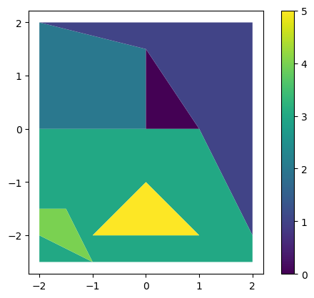
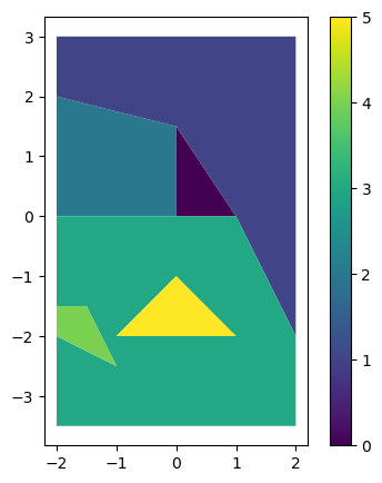
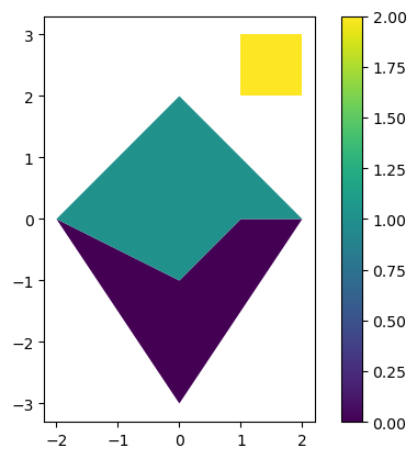
When no line ends on a given border, it is possible to modify this border’s position by specifying one of two parameters: - the buffer: enlarge the map by a given value on every border possible, unless a bbox is given. - bbox: coordinates of left, down, right, up: applied where possible. The coordinates cannot be inside the map.
[19]:
poly_map = line_map.to_poly_map(buffer=1)
poly_map.plot(legend=True, figsize=(5, 5))
[19]:
<Axes: >
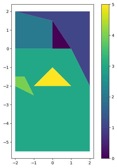
[20]:
original_borders = line_map.total_bounds
my_bbox = original_borders + [0, -3, 0, 0]
print(f"Intrisic borders:\n{original_borders}\nNew borders:\n{my_bbox}")

poly_map = line_map.to_poly_map(bbox=my_bbox)
poly_map.plot(legend=True, figsize=(7, 7))
Intrisic borders:
[-2.  -2.5  2.   2. ]
New borders:
[-2.  -5.5  2.   2. ]
[20]:
<Axes: >
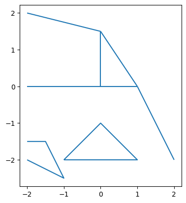
Polygons to lines
We can convert the geodataframe back to lines as follow:
[21]:
line_map = poly_map.to_line_map(apply_background_lc_id=False)
line_map.plot()
line_map.line_gdf
[21]:
| geometry | id_left | id_right | |
|---|---|---|---|
| index | |||
| 0 | LINESTRING (0.00000 0.00000, 0.00000 1.50000) | 2 | 0 |
| 1 | LINESTRING (0.00000 1.50000, -2.00000 2.00000) | 2 | 1 |
| 2 | LINESTRING (-2.00000 0.00000, 0.00000 0.00000) | 2 | 3 |
| 3 | LINESTRING (0.00000 0.00000, 1.00000 0.00000) | 0 | 3 |
| 4 | LINESTRING (1.00000 0.00000, 0.00000 1.50000) | 0 | 1 |
| 5 | LINESTRING (1.00000 0.00000, 2.00000 -2.00000) | 1 | 3 |
| 6 | LINESTRING (-2.00000 -1.50000, -1.50000 -1.500... | 3 | 4 |
| 7 | LINESTRING (-1.00000 -2.00000, 0.00000 -1.0000... | 3 | 5 |
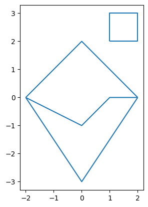
In the previous case we start with a full square map, but it is also possible to get the lines from polygons in an empty map. In that case, you can give the background landcover id when you instantiate the object.
[22]:
points = [
    [(-2, 0), (0, -3), (2, 0), (1, 0), (0, -1)],
    [(2, 0), (1, 0), (0, -1), (-2, 0), (0, 2)],
    [(1, 2), (1, 3), (2, 3), (2, 2)],
]
polygons = [Polygon(p) for p in points]
gdf2 = gpd.GeoDataFrame({"geometry": polygons, "id": [0, 1, 2]})
poly_map = PolygonMap(gdf2, background_lc_id=4)
poly_map.plot(legend=True)
[22]:
<Axes: >
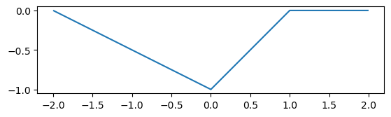
By default, only a single line will be drawn here separating the 0 and 1 values. This is because the value on the outside of the polygons, the white space, is not defined.
[23]:
poly_map.to_line_map().plot()
However, if we set apply_background_lc_id=True, all of the lines will be drawn, as the background_lc_id of the PolygonMap will be used as the value for the white-space.
[24]:
poly_map.to_line_map(apply_background_lc_id=True).plot()
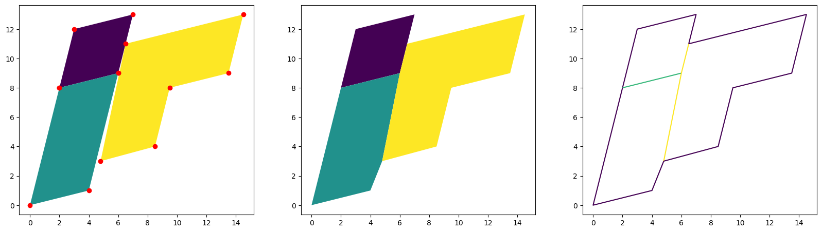
Polygons completion
Sometimes the polygons are not perfectly adjacent to each other, or vertices are missing, i.e a point appears in one polygon, but not on the adjacent polygon.
Examples of vertices mismatch: the points (4.8, 3) (the most obvious), (6, 9) (not part of the yellow polygon) and (6.5, 11) (not part of the purple polygon) on the figure below.
Arguments to use: If the vertices do not match, you will need to set the complete_polys to True when making the conversion. In that case, it is recommended to set atol to a small positive value for robustness. If the polygon are only misplaced use atol with an appropriate value for robustness. Neither are used by default.
Modified dataframe: If you use complete_polys and you want to access the modified dataframe, set return_polys_map to True. You will get two maps instead of one: the line map and the modified polygon map.
Efficiency: Using complete_polys will significantly increase the time needed. atol does not.
[25]:
tolerance = 1

points = [
    [(7, 13), (3, 12), (2, 8), (6, 9)],
    [(2, 8), (0, 0), (4, 1), (6, 9)],
    [(4.8, 3), (8.5, 4), (9.5, 8), (13.5, 9), (14.5, 13), (6.5, 11)],
]
polys = [Polygon(ls) for ls in points]
polys = gpd.GeoDataFrame({"geometry": polys, "id": [0, 1, 2]})
poly_map = PolygonMap(polys, background_lc_id=-1)

fig, ax = plt.subplots(1, 3, figsize=(20, 10))
poly_map.plot(ax=ax[0]);
for p in np.concatenate(points, axis=0):
    ax[0].plot(p[0], p[1], 'ro')


line_map, completed_poly_map = poly_map.to_line_map(
    apply_background_lc_id=True,
    atol=tolerance,
    complete_polys=True,
    return_poly_map=True
)
line_map.plot(color_lines="right", ax=ax[2])
completed_poly_map.plot(ax=ax[1]);
Colors
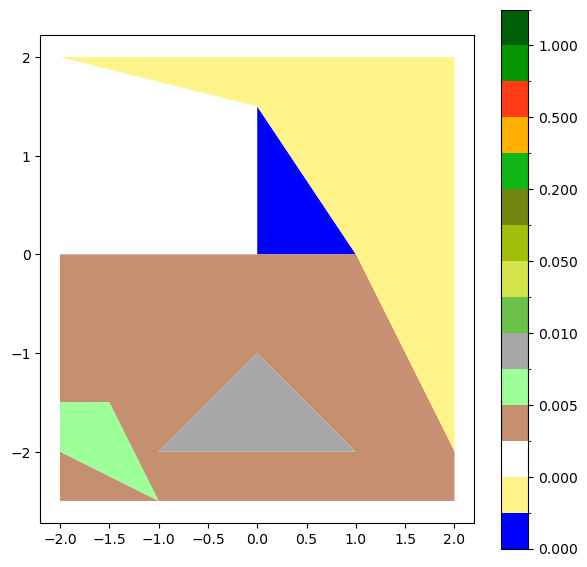
It is possible to plot the roughness values instead of the indices by specifying a color table.
The package include a colormap that will be used when using roughness values if no cmap or norm is specified.
[26]:
ids = list(range(6))

z0 = [
        0,
        0.0002,
        0.0003,
        0.001,
        0.005,
        0.008,
    ]

descriptions = [
    "Water",
    "Sand",
    "Snow",
    "Bare soil",
    "Mown grass",
    "Airport Runway",
]

landcover_table = LandCoverTable({
    i: dict(
        z0=z0[i],
        desc=descriptions[i],
        d=0.0,
    )
    for i in ids
})
[27]:
geo = [
    LineString([(0, 0), (0, 1.5)]),
    LineString([(0, 1.5), (1, 0)]),
    LineString([(1, 0), (0, 0)]),
    LineString([(0, 0), (-2, 0)]),
    LineString([(0, 1.5), (-2, 2)]),
    LineString([(1, 0), (2, -2)]),
    LineString([(-2, -1.5), (-1.5, -1.5), (-1, -2.5), (-2, -2)]),
    LineString([(-1, -2), (1, -2), (0, -1), (-1, -2)]),
]
id_left = [2, 1, 3, 3, 2, 1, 3, 5]
id_right = [0, 0, 0, 2, 1, 3, 4, 3]

gdf1 = gpd.GeoDataFrame({"geometry": geo, "id_left": id_left, "id_right": id_right})
line_map = LineMap(gdf1)
poly_map = line_map.to_poly_map()
poly_map.plot(legend=True, landcover_table=landcover_table, figsize=(7, 7))
[27]:
<Axes: >
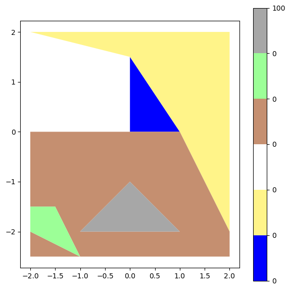
It is also possible to specify the colors when plotting or to store the colors in the landcover table.
[28]:
levels = [
    0,
    0.0002,
    0.0003,
    0.001,
    0.005,
    0.008,
    0.01,
    0.03,
    0.05,
    0.1,
    0.2,
    0.4,
    0.5,
    0.8,
    1,
    100,
]
colors = [
    (0, 0, 255),
    (255, 244, 137),
    (255, 255, 255),
    (197, 143, 112),
    (156, 255, 151),
    (167, 167, 167),
    (108, 193, 75),
    (213, 228, 75),
    (161, 191, 11),
    (114, 133, 17),
    (16, 182, 19),
    (255, 175, 1),
    (255, 60, 21),
    (5, 151, 0),
    (0, 95, 9),
]

landcover_table = LandCoverTable(
    {
        i: dict(
            z0=z0[i],
            desc=descriptions[i],
            d=0.0,
        )
        for i in ids

    },
    levels=levels,
    colors=colors,
)
landcover_table
---------------------------------------------------------------------------
AttributeError                            Traceback (most recent call last)
Cell In[28], line 37
      1 levels = [
      2     0,
      3     0.0002,
   (...)
     17     100,
     18 ]
     19 colors = [
     20     (0, 0, 255),
     21     (255, 244, 137),
   (...)
     34     (0, 95, 9),
     35 ]
---> 37 landcover_table = LandCoverTable(
     38     {
     39         i: dict(
     40             z0=z0[i],
     41             desc=descriptions[i],
     42             d=0.0,
     43         )
     44         for i in ids
     45
     46     },
     47     levels=levels,
     48     colors=colors,
     49 )
     50 landcover_table

File ~/projects/pywasp/modules/windkit/windkit/landcover.py:115, in LandCoverTable.__init__(self, levels, colors, *args, **kwargs)
    113 if colors == "default":
    114     colors = None
--> 115 self.add_colors_to_table(levels, colors)

AttributeError: 'dict' object has no attribute 'add_colors_to_table'
[ ]:
poly_map.plot(legend=True, landcover_table=landcover_table, figsize=(7, 7))
<Axes: >
[ ]: