RUNE validation

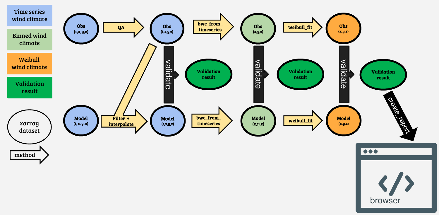
This note book demonstrates a validation of the different type of wind resource data formats. These formats were measured during the RUNE campaign in the winter of 2016 in Jutland, Denmark. The data are freely available as part of a paper that is available in the references at the end of this notebook. We start with a observed time series of wind speed and wind direction (obs) that have dimension time and coordinates x,y,z, which in windkit have been given the following names: west_east, south_north, height. The quality assurance of the observations and the extraction of the closest grid point (or interpolation to the mast position) is assumed to be done by the user. In other words, observations must be spatially and temporally aligned, i.e. dimension time, west_east, south_north, height must be the same on obs and model.

We import the xarray package for opening of example datasets

import xarray as xr
import os
import wind_validation as wv
from windkit.spatial import reproject, get_crs
from windkit import bwc_from_timeseries

Adding and filtering of data

We open a xarray dataset with lidar observations from the RUNE measuring campaign, rune_lidar. It contains wind speed and wind direction time series from 105 different points near the west coast of Jutland in an interval of 10 min. The variable ‘point’ contains the ID’s of the different points in the dataset and is not needed for further processing and therefore dropped.

rune_lidar = xr.open_dataset("data/dual_doppler.nc").drop_vars('point')

The other dataset rune_wrf_original is output of the flow from the WRF model. As can be seen in the paper, many different version of the WRF model were run during the RUNE project, but here we initially load the coarsest resolution from the YSU PBL scheme. Only a transect of the WRF simulations is loaded here.

rune_wrf_original = xr.open_dataset("data/FNL_YSU_COR_DMI_18km_transect.nc")

The model output is available every half hour and the grid spacing of this WRF setup was 2 km. Therefore we have to make sure that the model and observations have the same format. First we have to reproject the WRF output so that is uses the same metric coordinate reference system (CRS) as the observations. This is achieved by obtaining the CRS from the observations using the get_crs method and then reprojecting the data set with reproject. Subsequently, we obtaind the nearest points from the WRF simulations at each point of the lidar observation using the nearest_points method.

from windkit.spatial import nearest_points
rune_wrf = reproject(rune_wrf_original, get_crs(rune_lidar))
rune_wrf = nearest_points(rune_wrf, rune_lidar)
rune_wrf = rune_wrf.rename({"WSPD":"wind_speed","WDRO":"wind_direction"})

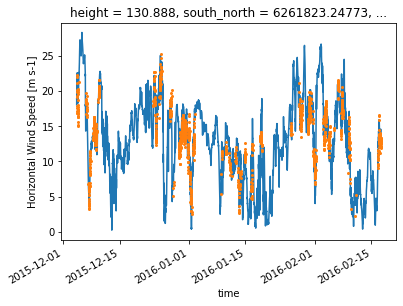
We can plot one point (nr 100) from the dataset and obtain a time series to study the behaviour of the wind over the 4 month measurements campaign. We can see that the lidar (orange points in the plot below) was only operating some of the time.

rune_wrf["wind_speed"].isel(point=100).plot()
rune_lidar["wind_speed"].isel(point=100).plot(marker='o',linewidth=0,markersize=2)

[<matplotlib.lines.Line2D at 0x7f887b8a1220>]

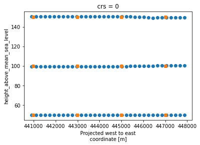
To understand the position of each of the measuring points of the lidar we can plot the different positions in the transect across the coast (blue points). The WRF output has a rather coarse resolution of 3 km (orange points). Note that the y-axis shows the height abve sea level, so when we are over land the apparent measuring height is closer to the surface.

rune_lidar.plot.scatter("west_east","height_above_mean_sea_level")
rune_wrf.plot.scatter("west_east","height_above_mean_sea_level")

<matplotlib.collections.PathCollection at 0x7f887b8a1790>

Because the model output and measurements will generally not be at exact same time steps, we interpolate the WRF time series linearly using the time stamps from the lidar data, so that we have the same number of samples in both datasets.

rune_wrf = rune_wrf.interp_like(rune_lidar['time'], method='linear')

From time series to histogram

To convert time series to a histogram we can use the bwc (binned wind climate) from time series method from windkit. The normalize keyword is set to false, so we retain the original counts per bin, whereas setting it to true would normalize each sector with the number of observations in that sector. The wind direction frequencies are then lost and they are therefore stored in a variable wdfreq.

his_lidar = bwc_from_timeseries(rune_lidar, normalize=False)
his_wrf = bwc_from_timeseries(rune_wrf, normalize=False)

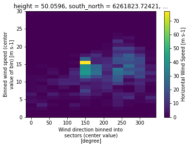
We can plot the wind vector count and visualize. The plot contains a count per cell along the dimensions wind speed and wind direction. Wind directions are denoted by the center value of 30 degree wide bins, where the first bin is centered for winds from the North (0 degrees). The wind direction is increasing in clockwise direction.

his_lidar.isel(point=0)['wv_count'].plot()

<matplotlib.collections.QuadMesh at 0x7f887a8db040>

We can validate a time series by doing a time series validation with the validate method. The wind validation package will automatically detect the data structure and select the statistics and metrics that can operate on that data structure. By default the validation works with a standard set of statistics and metrics (denoted with basic). This can be changed by modifying the keyword arguments metrics and stats.

results = wv.validate(rune_lidar,rune_wrf,metrics="basic",stats="basic")

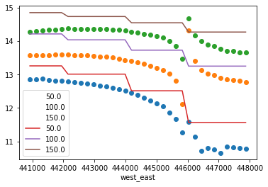
We can now plot the mean wind speeds from the RUNE dataset and compare with the WRF output. Below, the observations are plotted as points, and the output from the WRF grid cells is denoted with lines. The three different heights at which measurements were available are shown. The WRF model has a gridspacing of 3 km, so the wind speeds look like step functions for the model.

import matplotlib.pyplot as plt
plotres = results.to_dataframe().set_index('west_east')
plotres.groupby('height_above_mean_sea_level')['obs_wind_speed_mean'].plot(marker='o',linewidth=0,legend=True)
plotres.groupby('height_above_mean_sea_level')['mod_wind_speed_mean'].plot(legend=True)

height_above_mean_sea_level
50.0     AxesSubplot(0.125,0.125;0.775x0.755)
100.0    AxesSubplot(0.125,0.125;0.775x0.755)
150.0    AxesSubplot(0.125,0.125;0.775x0.755)
Name: mod_wind_speed_mean, dtype: object

For a validation of a histogram we call validate again, but this time using the histograms as input:

results_his = wv.validate(his_lidar, his_wrf, stats="basic", metrics="basic")

We can see the call looks exactly the same, apart from the input. The basic stats and metrics are used in this example. If you want to calculate the Earth Movers Distance (EMD) you can specify to calculate all available metrics & statistics instead of the basic ones. This requires you to install the pyemd package, which most easily installed using conda.

tmp_his = wv.validate(rune_lidar, rune_wrf, stats="all", metrics="all")

However in some cases (such as better performance) it might be useful to get only specific stats & metrics. This can be achieved by selecting explicitly the stats & metrics. You can read the documentation to get a full list of available options. To calculate only the mean error in wind speed and power density, you can fo for example:

tmp_his = wv.validate(his_lidar, his_wrf,
    stats=[
        # (variable,stat)
        ("wind_speed","mean"),
        ("power_density","mean")
    ],
    metrics=[
        # ((variable,stat), metric)
        (("wind_speed","mean"),"me"),
        (("power_density","mean"),"me")
    ])

To create a report we can convert the results to a dataframe and call create_report. This will open an html file in your browser where you can study the comparison in more detail.

wv.create_report(results, obs_name="RUNE experiment", mod_name="RUNE WRF output")  # opens up the report in the browser

HTML report saved in: /tmp/tmpsn2ac_wz.html

Creating a report from the histogram validation results works exactly the same, but we pass in the results_his dataset. Alternatively you can save the html file to your desired location (please make sure that the directory exists):

dir = os.path.dirname(os.path.realpath("__file__")) # just as an example save it to the notebook directory
wv.create_report(results_his, obs_name="RUNE experiment", mod_name="RUNE WRF output", dest=dir + "/report.html")

HTML report saved in: /home/neda-ubuntu/DTU/repo/wind-validation/docs/source/report.html

Comparison of models in one report

During the RUNE campaign a range of WRF simulations were performed. We can pass multiple validation results to the reporting function so that we can compare how different models perform on the same set of observations. For instance, let’s use the the WRF simulations with a different PBL scheme. The original simulations that we compared with were performed using the YSU scheme. However, also the MYJ scheme was used to simulate the RUNE campaign. The MYJ scheme is a 1.5 order closure scheme compared to the 1st order YSU scheme. Note that we take the same steps as before to align the data with the observations in both space and time.

rune_wrf_myj = xr.open_dataset("data/FNL_MYJ_COR_DMI_18km_transect.nc")
rune_wrf_myj = reproject(rune_wrf_myj, get_crs(rune_lidar))
rune_wrf_myj = nearest_points(rune_wrf_myj, rune_lidar)
rune_wrf_myj = rune_wrf_myj.rename({"WSPD":"wind_speed","WDRO":"wind_direction"})
rune_wrf_myj = rune_wrf_myj.interp_like(rune_lidar['time'], method='linear')
results_myj = wv.validate(rune_lidar,rune_wrf_myj,metrics="basic",stats="basic")

validations = [results,results_myj]
obs_names = ["RUNE experiment", "RUNE experiment"]
mod_names = ["RUNE WRF YSU", "RUNE WRF MYJ"]
wv.create_report(
    validations,
    show=True,
    obs_name=obs_names, # here the names are required!
    mod_name=mod_names, # here the names are required!
    #dest="/mnt/c/Users/rogge/Desktop/comp.html"
) # opens your browser :)

HTML report saved in: /tmp/tmp1ajp9zah.html

References

Floors, R., Hahmann, A. N., & Peña, A. (2018). Evaluating Mesoscale Simulations of the Coastal Flow Using Lidar Measurements. Journal of Geophysical Research: Atmospheres, 123(5), 2718–2736. https://doi.org/10.1002/2017JD027504

Floors, R. (2017). Files with RUNE experiment measurements and WRF modelling results. https://doi.org/10.5281/zenodo.834591